ML-driven Alpha Search and Alpha Allocation on Large Scale Part II: Alpha Search on Large Scale

Summary of the talk given at the Bloomberg Quantamental Exchange 2023
The series on the topic ‘ML-driven Alpha Search and Alpha Allocation on Large Scale’ consists of the following 3 sections.
Part 1: Recent Trends in Machine Learning
Part 2: Alpha Search on Large Scale
Part 3: Enhanced Alpha Search and Strategy Allocation on Large Scale
In this section, we will explore the search for investment strategies with excess returns (alphas) on large scale.
Introduction to Alpha Search
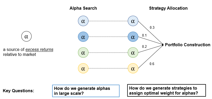
Alpha search is to find sources of excess returns relative to market. We will specifically look into two aspects of alpha search namely:
1) How do we find sources of excess returns in today's world where the amount of data available is increasing exponentially?
2) Given that we have found a way of finding alphas, how do we accomplish so on large scale?
Alpha Generation
Simple Example
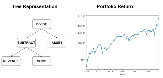
In Figure 10 shown below, we have a quality factor – an alpha that is commonly known amongst quantitative researchers. The calculation of the quality factor is a straightforward process of dividing gross profit by assets. The performance of the final portfolio can then be evaluated simply by taking, for instance, long positions on the companies with positive values and taking short positions on the companies with negative values as shown by the graph on the figure.
Generalized Steps
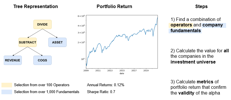
We can provide a more detailed and generalized description of formulating a factor by analyzing each step at a greater depth. When we are formulating a factor, we are essentially finding a combination of mathematical operators and company fundamentals. In a broader sense, a value factor is formed by opting for “Divide” and “Subtract” out of many other possible mathematical operators like “Add” and “Multiply” and by selecting “Revenue”, “Cost of Good & Services” and “Asset” out of many other possible company fundamentals like “Cash Flow”, “Net Debt” and “Earnings”. For a given investment universe, for instance, all those companies listed on the NYSE, NASDAQ, and AMEX and a certain date range, the process involves calculating the factor for all the companies in the universe. After evaluating the long-short portfolio of the factor, we can compute a set of metrics such as annual returns and sharpe ratio to determine the validity of the factor as an alpha.
From Expressions to Markov Chain Monte Carlo
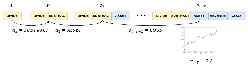
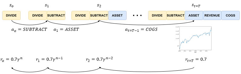
Going a step further, the generalized steps of formulating a factor can be represented as a Markov Chain. I’ll try to make the explanation easier by making an analogy to a game of chess. A state is equivalent to the chess board, the result of all the actions that have been taken in the past. By taking an action a zero of “subtract”, which is equivalent to moving a horse in chess, we now make a transition from s0 to a new state s1 in Figure 12.
Eventually, we reach a stage where a factor is completed just as a game of chess has its end. Once the factor is completed, we can the portfolio metric in this case the sharpe ratio, in the same way, that the outcome of a chess game can be determined as a win, a draw, or a loss. This is known as the reward, a numerical representation of how “good” a state is.
What we now want to do is to evaluate every state. This is comparable to assessing how “good” the state is, how likely I am going to win the game of chess in the middle of the game, or how likely I am going to construct an alpha. In the middle of the game or in the middle of making a factor, however, it is often difficult to evaluate the state for two reasons:
1) We are dealing with spare rewards setting where a reward can only be calculated once the factor is complete or once the game is complete.
2) We are dealing with discrete rewards setting where we want to focus on achieving the long-term goal of winning the game and creating an alpha rather than achieving any intermediate steps that may not be relevant to the final outcome.
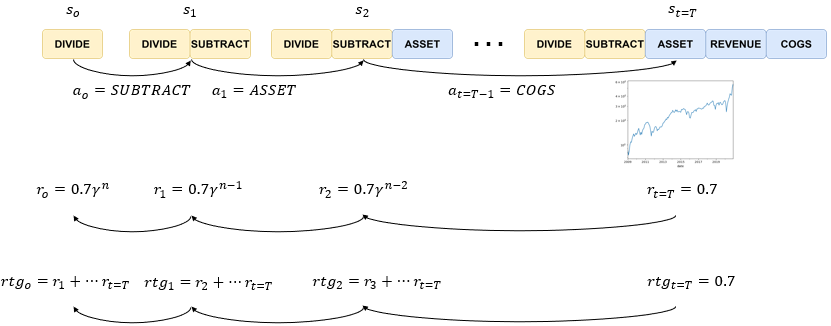
To address the first issue of spare rewards, we approximate the reward by using a discounted reward function that multiplies the discount rate for every deviation from final time t=T. As shown on the slide r two is equal to 0.7 times the discount rate to the power of n-2, r one is equal to 0.7 times the discount rate to the power of n-1 and etcetera.
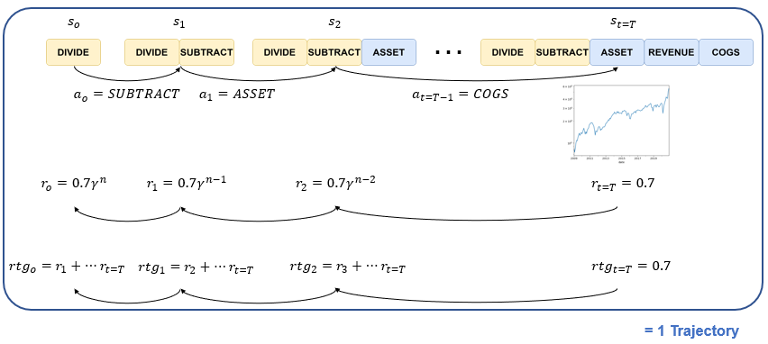
To resolve the second issue of discrete rewards, we then calculate what is known as rewards-to-go which is simply the sum of all future rewards. Rtg0 at step t=0 is the sum of r one to r T, and rtg1 at step t=1 is equal to the sum of r2to rT. Reward-to-go is a greater assessment of how good a state is because it takes into account the potential of the current state to earn all future rewards until the end of the episode rather than just a single reward at a current timestep.
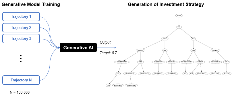
Now that we have a set of states, actions, and rewards-to-go for all timesteps, we have one complete trajectory. The same process can be applied to other known factors like momentum, growth, and quality factors as well as those previously unseen factors to gather hundreds of thousands of trajectories.
These trajectories can then be used to train generative models to learn about the combination of mathematical operators and company fundamentals that are more likely to qualify as an alpha. Once the training is complete, the model can start to generate factors from complete blank to one that is more likely to yield our desired portfolio metric. The diagram on the right shows our trained generative model that is in the process of formulating a factor.
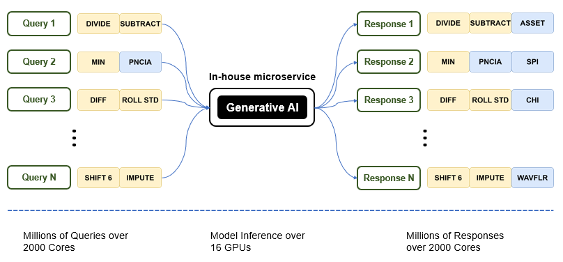
Deployment on Large Scale
The next question is then how do we deploy the model that we have developed on large scale. A key aspect to consider is that the input going into the model is just the current state, a relatively simple query that can be made over CPUs. The model makes a more efficient inference over GPUs than over CPUs to suggest the next optimal action – in the first case being ASSET, the next case being SPI, and CHI and etcetera. Taking these aspects into consideration, one can create an asynchronous microservice to place the generative models online with GPUs, and return output for each query made by each CPU one at a time. The notion of creating an in-house microservice, therefore, utilizes the available computing resources at a maximum capacity.
In the subsequent section, I will be talking about additional considerations for alpha search and generation of strategy allocation!
Thank you for your time and for those who are interested in learning more about Akros Technologies, you can contact us via email and here are a few links you could refer to!